Back to Hans Lundmark's Complex analysis page.
The theory of elliptic functions is one of the highlights of 19th century complex analysis, connected to names such as Gauss, Abel, Jacobi, and Weierstrass. This page barely scratches the surface of the theory, but maybe the pictures here can serve as a gentle introduction. At least for me, seeing these pictures made elliptic functions seem less scary than what I thought they were.
Before we look at elliptic functions, let's recall what we know about our dear old friend the sine function. To begin with, it is periodic with period 2π, and analytic in the whole complex plane (there are no poles or other singularities).
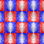
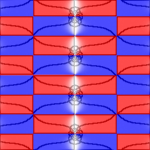
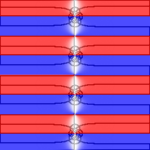
Below are two domain coloring plots using different coloring schemes, both showing w = sin(z) on the square with corners at z = ±6±6i :
The first plot uses my standard coloring, as explained elsewhere on this site (see the main page).
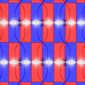
In the second plot, the grid is more emphasized, while the shading based on absolute value is removed. Blue (red) color indicates regions mapped to the upper (lower) half plane. These regions are “half-strips”; the upper ones continue upwards forever, while the lower ones continue downwards forever. They are π units wide, and have corners at the points where the function's derivative cos(z) is zero (that is, at odd multiples of π/2). Except at these points, the mapping is conformal – notice how the grid lines intersect at right angles.
Make sure that you can trace how the function grows from sin(z) = 0 at z = 0 (start at the center of the picture) to sin(z) = 1 at z = π/2 (the first corner as you move to the right from there).
Then if you continue moving to the right, the function decreases to sin(z) = 0 again, then further down to sin(z) = −1, then up, etc.
On the other hand, if you instead turn 90 degrees at the corner and continue upwards (or downwards) along the line z = π/2+iy, then the function continues to grow; you will pass grid line intersections corresponding to sin(z) = 2, 3, 4, 5, etc.
In the interior of the blue/red regions, the sine function assumes complex values. For example, if you follow the grid line leading “north-west” from that same corner at z = π/2, you will first come to a grid line intersection at the point z where sin(z) = 1 + i, next to the intersection where sin(z) = 1 + 2i, and so on.
Now we are ready to look at our first elliptic function, a function named sinus amplitudinis (the sine of the amplitude) by Jacobi in his famous work Fundamenta nova theoriae functionum ellipticarum (New Foundations of the Theory of Elliptic Functions) from 1829. It is denoted by sn(z,k) and depends on a parameter k which is called the “modulus”. (Note: sometimes m = k2 is called the modulus instead.)
Usually k is taken between 0 and 1, but the function can also be defined for complex values of k. When k = 0, sn(z,k) simply reduces to sin(z), so it can be thought of as a “distorted sine function”.
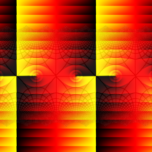
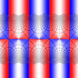
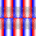
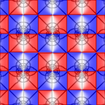
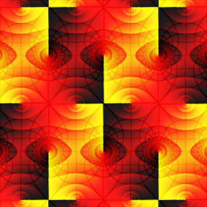
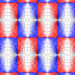
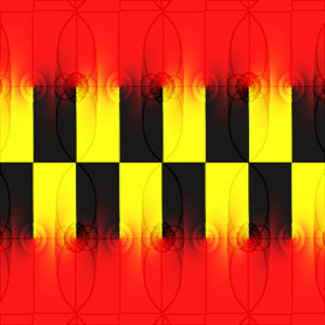
Here is what the function looks like when k = 1/4, again on the square with corners at z = ±6±6i :
Along the real axis (the middle horizontal line in the plot), this function looks much like the sine function; it oscillates periodically between −1 and 1. The period depends on k and is actually larger than 2π, although for k = 1/4 the difference is so small that it's barely noticable in the picture.
In the complex plane, however, something new has happened: the vertical edges of the half-strips have bent inward to enclose rectangles instead. Where the tips meet, the function has simple poles. The function is doubly periodic; it repeats itself not only in the right-left direction, but in the up-down direction as well.
The general definition of an elliptic function is a function F(z) that is meromorphic and doubly periodic. Meromorphic means analytic except possibly at isolated poles, and doubly periodic means that there are two periods A and B (complex numbers) such that F(z+nA+mB) = F(z) for all z∈C and all integers n and m. The periods span a parallelogram in the complex plane. If F(z) is known in this parallelogram, then it is known everywhere because of the periodicity. In the case of sn(z,k) with 0<k<1, A is real, B is purely imaginary, and the period parallelogram is made up of two blue and two red rectangles.
The sine function w = sin(z) is the inverse of z = arcsin(w), which is an antiderivative of 1/√[1−w2]. This can be taken as the definition of the sine function, except that it only provides half a period; the function has to be extended to the whole complex plane by symmetry and periodicity.
Similarly, Jacobi's elliptic function w = sn(z,k) can be defined as the inverse function of a particular antiderivative of 1/√[(1−w2)(1−k2w2)], with the understanding that it should be extended to the whole complex plane in a suitable way.
[The antiderivative of 1/√[(1−w2)(1−k2w2)] cannot be expressed in terms of elementary functions – that's why new functions like sn appear in this context. Integrals involving square roots of cubic or quartic polynomials are called elliptic integrals, because a particular such integral arises when computing the arc length of an ellipse. Elliptic integrals were studied for over a century before anyone thought of looking at their inverses, which then became known as “elliptic” functions.]
An equivalent definition is to say that w = sin(z) is the solution of the differential equation (dw/dz)2 = 1−w2 and that w = sn(z,k) is the solution of the differential equation (dw/dz)2 = (1−w2)(1−k2w2), in both cases with initial conditions w = 0, dw/dz = 1 at z = 0.
From these differential equations, we see that in both cases the derivative dw/dz is zero when w = ±1. But in the elliptic case, the derivative is zero also when w = ±1/k, and this produces the additional corners that aren't present in the trigonometric case. Look back at the plot of w = sn(z,1/4) above, and check using the grid that the “new” corners indeed occured at the points where w = ±1/k = ±4.
Now look at the differential equations for real values of the variable z. If we suppose that 0 < k < 1, then the derivative dw/dz first becomes zero when w = 1 (since 1 is less than 1/k). This means that for real z the solutions oscillate periodically between −1 and +1. But the extra factor (1−k2w2) makes the derivate smaller in the elliptic case than in the trigonometric case, so the elliptic functions oscillate slower (the larger k is, the slower the oscillation).
The trig functions have period 2π, so one quarter of a period equals π/2; this is how long it takes for sin(z) to grow from 0 to 1, and it equals the integral of 1/√[1−w2] from w = 0 to w = 1.
Similarly, how long it takes for sn(z,k) to grow from 0 to 1 is determined by the integral of 1/√[(1−w2)(1−k2w2)] from w = 0 to w = 1. This value is denoted by K(k), and it increases from π/2 to infinity as k increases from 0 to 1. Even though the integral defining K(k) can't be expressed in terms of elementary functions, there is an amazingly simple and efficient formula for computing it: K(k) = (π/2) / AGM(1,k′), where k′ = √[1−k2] and AGM(a,b) denotes the arithmetic-geometric mean of a and b. This idea goes back to Lagrange in 1785, and has recently led to some of the best currently known algorithms for computing π. Similar methods can also be used for computing the sn function itself.
The number K(k) is half the width of the rectangles in the plot, and the right-left period of the sn function is consequently 4K(k).
If we allow z to be complex, and take off in the vertical direction from z =K(k), then the time it takes for the function to grow from 1 to 1/k is given by the integral of 1/√[(w2−1)(1−k2w2)] from w = 1 to w = 1/k. This value is denoted by K′(k) and happens to be the same as K(k′). This is the height of the rectangles in the plot, and the up-down period of the sn function is consequently 2iK′(k).
(Note: The primes in K′ and k′ have nothing to do with derivatives.)
The plots below show w = sn(z,k) for the following ten values of k: 0, 0.02, 0.05, 0.1, 0.2, 0.5, 0.9, 0.95, 0.99, 1. When k = 1, the real period goes to infinity and sn(z,k) reduces to tanh(z), which only has the purely imaginary period iπ.
The Jacobi sn function appears, for example, in the solution of the pendulum equation d2θ/dt2+ω2sin(θ) = 0. For small oscillations, the approximation sin(θ) ≈ θ reduces this equation to the harmonic oscillator, with trig solutions of period 2π/ω. Here is a quick sketch of how to derive the exact solution, without the approximation of small oscillations. Assume for simplicity that the energy is low enough that the pendulum doesn't swing past the upright position, so that there is a maximal angle θmax∈[0,π], and assume also that θ = 0 when t = 0. Let z = ωt. Then d2θ/dz2+sin(θ) = 0. Multiply this equation by dθ/dz and integrate: (1/2)(dθ/dz)2−cos(θ) = E, where E = −cos(θmax) = 2k2−1, if we define k = sin(θmax/2)∈[0,1]. Then w(z) = (1/k) sin(θ(z)/2) will satisfy the defining differential equation for the sn function (including initial conditions), so that w(z) = sn(z,k). Consequently, the solution of the pendulum equation is θ(t) = 2 arcsin[k sn(ωt,k)].
When k = 0 the pendulum just hangs straight down without moving, while the case k = 1 is a pendulum which performs a single swing between upright positions in the limits t→±∞. The larger the modulus k, the larger the period 4K(k)/ω and the amplitude θmax = 2 arcsin(k).
The cosinus amplitudinis function cn(z,k) is defined by the same differential equation as sn, but with initial conditions w = 1 and dw/dz = 0 at z = 0. The functions sn and cn satisfy the identity cn2 + sn2 = 1. There is also a third Jacobian elliptic function dn(z,k), which is defined such that dn2 + k2sn2 = 1. These three functions satisfy gazillions of identities which all look like trigonometric formulas running amok. See MathWorld: Jacobi Elliptic Functions for a sample.
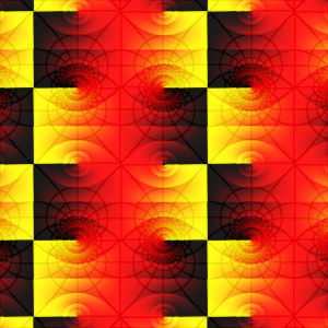
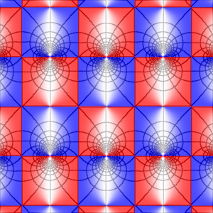
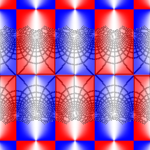
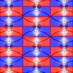
Below are plots of cn(z,1/4). Corners at z = ±6±6i as usual. The periods of cn are 4K(k) and 2K(k)+2iK′(k).
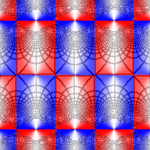
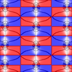
And here is dn(z,1/4). The periods of dn are 2K(k) and 4iK′(k). On the real axis the function is positive (it oscillates between k′ and 1), but it has complex zeros (and poles).
We see that the three Jacobian functions sn, cn, dn have the periods 4K(k) and 4iK′(k) in common, although in each case these are not the smallest periods possible.
The lemniscate is the famous curve that looks like the infinity symbol ∞. It is the image of the hyperbola x2−y2 = 1 under inversion with respect to the unit circle x2+y2 = 1, and its equation in polar coordinates (r,φ) is r2 = cos(2φ).
A fun but somewhat unorthodox way of drawing the lemniscate is to make a domain coloring plot of w = (4/π) arcsin(1/z√2). Abracadabra – there it is:
[This works since s = √2 sin(w) maps Cartesian grid lines to ellipses and hyperbolas which have their focal points at ±√2 (like x2−y2 = 1), and z = 1/s is inversion in the unit circle followed by complex conjugation. Hence w = arcsin(1/z√2) maps the lemniscate onto some grid lines, and the constant 4/π is only there to make these grid lines exactly w = ±1+iy so that their preimages will be visible in the plot.]
It is a routine calculus exercise to show that the arc length, call it z, of a part of the lemniscate which goes from the origin out to radius w ≤ 1 (in the first quadrant, say) is given by the integral of 1/√[1−r4] from r = 0 to r = w. This integral can't be expressed in elementary functions, so again we simply have to take it as the definition of a new function z = F(w). The inverse of this function, the sinus lemniscaticus denoted w = sinlemn(z) or w = sl(z), is the original elliptic function; Gauss discovered around 1797 that it is doubly periodic as a function of a complex variable.
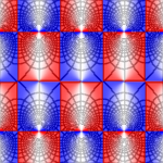
Since 1−w4 = (1−w2)(1−i2w2), we see that sinlemn is nothing but the Jacobi sn function with imaginary modulus: sinlemn(z) = sn(z,i), which actually turns out to equal cn(K(1/√2)−z√2,1/√2). This is what is looks like (corners at z = ±6±6i):
The width (and height!) of the rectangles is 2K(i)=2.622… which is the arc length of one loop of the lemniscate; that is, half the length of the whole curve. This value is known as the lemniscate constant. (Compare with π, which is half the length of the unit circle.)
Pick any (non-parallel) periods A and B. Put a translated copy of the function w = 1/z2 over each point nA+mB. Try to add them up. Unfortunately, this sum doesn't converge, but one can modify it a little (no details here) so that it converges to a doubly periodic function w = ℘(z; g2,g3) which has a double pole at each point nA+mB. This is Weierstrass's “p function”. According to tradition, the “p” should always be written with the fanciest font available! The two numbers g2 and g3 depend in an explicit way on the chosen periods A and B (but, again, no details here).
Note that the elliptic functions we've seen so far all had simple poles, two in each period parallelogram, whereas the ℘ function has one double pole in each period parallelogram instead.
The Weierstrass function w = ℘(z; g2,g3) satisfies the differential equation (dw/dz)2 = 4w3−g2w−g3.
You can read more at MathWorld: Weierstrass Elliptic Function and Wikipedia: Weierstrass's elliptic functions. Here, we'll just take a quick look at two particularly symmetric cases with impressive names.
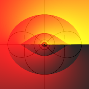
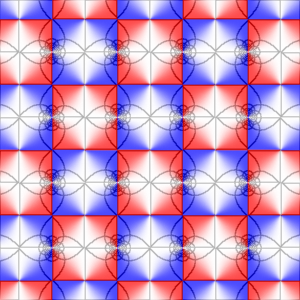
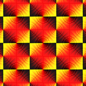
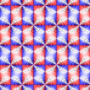
First, the lemniscatic case g2 = 1, g3 = 0, where the period parallelogram is a square, the length of whose diagonal is twice the lemniscate constant mentioned above. (As before, the corners of the plot are at z = ±6±6i.)
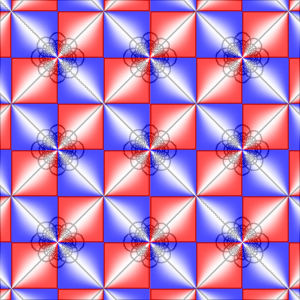
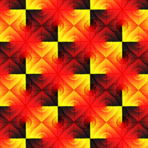
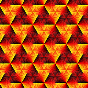
And, to finish off the show, the equianharmonic case g2 = 0, g3 = 1. Here the lattice is hexagonal, the period parallelogram being made up of two equilateral triangles of side 3.0599… (which is twice the ω2 constant):
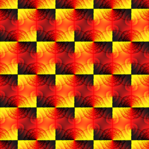
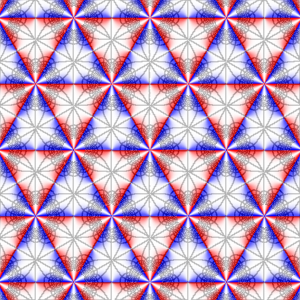
The triangles are more clearly visible in the plot of the derivative d℘/dz, which has triple poles at the lattice points:
Here are a few good books to read if you want to learn more:
Original version 2004-10-19. Last modified 2025-05-12. Hans Lundmark (hans.lundmark@liu.se)