Back to Hans Lundmark's Complex analysis page.

Taylor polynomials of the exponential function

Consider the exponential function e^z and its Taylor polynomials P_n(z) about z = 0 (also known as Maclaurin polynomials):

The series for e^z converges for all z∈C, so the polynomial P_n should be a very good approximation to e^z when n is large. But a polynomial of high degree has lots of zeros in the complex plane, while the exponential function has no zeros at all! Isn't this a bit strange?

Well, not really. A polynomial cannot possibly approximate e^z in the whole complex plane. For example, e^x grows faster than any polynomial as x tends to plus infinity along the real axis. So we should only expect P_n to approximate e^z in some region around the origin. The size of the region must grow when n grows, otherwise the Taylor series wouldn't converge for all z. But for any fixed n, P_n may very well have zeros outside this region of good approximation.

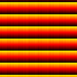
Recall the domain coloring plot of the exponential function, here shown on a square with corners at z = ±20±20i :

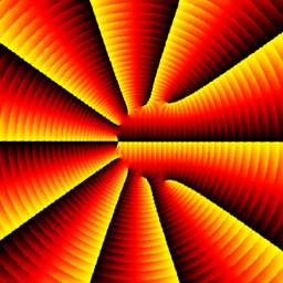
Now look at the plots (on the same square) of the Taylor polynomials P₅ , P₁₀ , P₁₅ , P₂₀ , and P₂₅ :

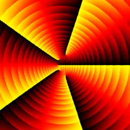
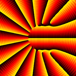
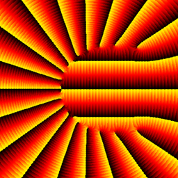
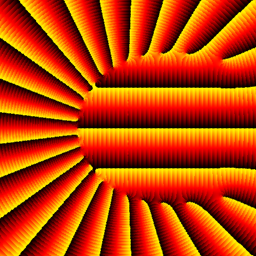
(Side note: Do you get the impression that these images are rotating? Then check out Akiyoshi's illusion pages for a mindboggling collection of similar optical illusions.)

As we anticipated, the zeros of P_n move further and further away from the origin as n increases. There is a region in the middle where the polynomials indeed look like e^z, but for large | z | the highest degree term zⁿ / n! dominates and the approximation breaks down.

The zeros of P_n(z) seem to be very regularly distributed, as if they lie along some smooth curve in the plane. To study this, it is convenient to shrink the picture of P_n by a factor of n, to keep the zeros from running off to infinity as n increases. In other words, one studies the zeros of Q_n(z) = P_n(nz).

Simple fact: The zeros of Q_n(z) lie in the unit disc | z | ≤ 1. (That is, the zeros of P_n lie in the disc | z | ≤ n.)

Proof: The coefficients of Q_n are positive and nondecreasing, since the coefficient of z^k is n/k times the coefficient of z^k−1 (we consider the constant term as the first coefficient here). Hence the "reversed" polynomial zⁿ Q_n(z⁻ⁿ) has positive and nonincreasing coefficients. The Eneström–Kakeya theorem says that such a polynomial has no zeros inside the unit circle. Done!

(Sketch of proof of the Eneström–Kakeya theorem: multiply the polynomial by z−1 and use the triangle inequality to show that the resulting polynomial is nonzero for | z | < 1.)

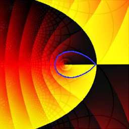
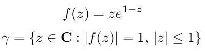
Deep fact (proved by Szegő in 1924): As n goes to infinity, the zeros of Q_n(z) accumulate on the curve γ shown in blue on the plot below (corners at z = ±2±2i):

Problems of this type are still an active research topic. One might study the rate of convergence, or how densely the zeros accumulate on different parts of the curve. (See for example the paper Zeros of the partial sums of cos (z) and sin (z). I by Richard S. Varga and Amos J. Carpenter, Numerical Algorithms 25: 363-375, 2000.)

Asymptotic behavior of orthogonal polynomials (and their zeros) is a closely related subject where powerful new techniques have been developed in recent years. Details about this can be found in the book Orthogonal Polynomials and Random Matrices: A Riemann-Hilbert Approach by Percy Deift.