Visualizing complex analytic functions using domain coloring
1 Introduction
The aim of this document is to illustrate graphically some of the striking
properties of
complex analytic functions (also known as
holomorphic functions).
Anyone can enjoy the pictures, of course,
but to appreciate their meaning you need to know some complex analysis.
A function
f :
R →
R is usually visualized by
drawing its graph
y =
f (
x ) in a coordinate system
with one axis for the domain variable
x and one axis for the range variable
y.
However, for complex functions
f :
C →
C
we run into trouble;
since the complex plane
C is two-dimensional,
we would need a four-dimensional space to draw the
graph
w =
f (
z ).
And since four dimensions are one too many for most ordinary mortals,
other techniques of visualization are called for.
The most common method is to draw two copies of the complex
plane, one for
z and one for
w, and then in the
w plane draw the
images under
f of various curves and regions in the
z plane.
This is very useful, but it can be difficult to capture in a single picture
what the function f really does.
This drawback can be at least partly overcome by a simple technique known as
domain coloring
(a term coined by professor Frank Farris).
It works as follows:
- "Paint" the w plane, either by copying a picture of something onto it,
or by using some formula to determine the color of each point.
- Color every point z in the domain of f with the color of the corresponding point w = f ( z ).
The resulting colored picture in the
z plane is the "graph" of the function
f.
This method is obviously very well suited for computer graphics.
Although domain coloring can be used to draw pictures of arbitrary
functions
f :
C →
C (or
R2 →
R2 ), I have only considered
analytic functions here, since they have some very interesting
properties which are clearly visible in the pictures. Here are some of
the things that will be illustrated:
- Behaviour near zeros, poles, branch cuts and essential singularities.
- Conformality (preservation of angles).
- Lucas' theorem on the critical points of a polynomial.
- Möbius transformations.
- Some common elementary functions.
- The argument principle.
- The maximum principle.
2 Domain coloring - a simple example
Let us take a closer look at how domain coloring works,
by considering an example: the squaring function
f (
z )=
z2.
The first thing to do is to choose a coloring of the
w plane.
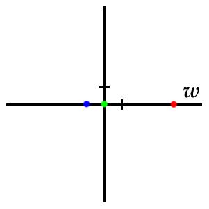
For the sake of example, our first coloring will be very simple:
let the point
w=4 be red, the point
w=−1 blue, the point
w=0 green,
and the rest of the
w plane white
(see figure
1, where the axes are shown for reference only; they don't belong to the coloring).
Figure 1:
A simple coloring of the
w plane
Now for each point in the
z plane we determine its color by
computing
w=
f (
z )=
z2 and looking at what color that point has in our
colored
w plane.
For example,
z=3 will be white,
since
f ( 3 )=3
2=9 and
w=9 is in the white region of the
w plane.
Obviously, with the coloring we have chosen, nearly every
z will be white.
The only points that will
not be white are
- z=± 2 which will be red, since w=f ( ± 2 )=22=4 is red,
- z=± i which will be blue, since w=f ( ± i )=i2=−1 is blue,
- z=0 which will be green, since w=f ( 0 )=02=0 is green.
Consequently, we obtain the picture shown in figure
2.
Figure 2:
The corresponding simple picture of
f (
z )=
z2.
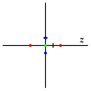
Note that the set of red points in the
z plane constitutes the inverse image (under the mapping
f)
of the set of red points
in the
w plane, and similarly for the other colors.
So instead of looking in the w plane at images of z points, as in the conventional technique,
we are looking in the z plane at inverse images of w points.
This has the advantage of giving a clear picture also of functions which are not one-to-one.
By using many colors, we can look at the inverse images of many points
(in principle, all of them) simultaneously.
Before we proceed,
let me also point out that if
f is the identity function,
f (
z )=
z,
then the picture in the
z plane will of course look exactly like the
coloring chosen in the
w plane.
3 Choosing the coloring
The coloring of figure
1 is of course too simple to be useful;
the only things that can be read off about the function
f (
z )=
z2
from figure
2
is where the values 4, −1, and 0 are assumed.
All other information about
f is lost in the great white void.
Let us try to find some better way of coloring the
w plane.
Obviously it is desirable that different points be easily distinguishable;
looking at a point in the
z plane,
it should be easy to find the corresponding point in the
w plane,
so that we quickly can identify the value of
f (
z ).
This is perhaps most easily accomplished by superimposing
an actual picture on the
w plane, since the brain easily identifies
features in a picture even if it's heavily distorted.
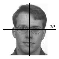
An example of this is shown in figure
3, which shows a picture of me
superimposed on a part of the
w plane,
and the corresponding picture of
f (
z )=
z2 in the
z plane.
The real and imaginary axes and the square with corners ± 1 ±
i are shown for reference
(the scale is not the same in the two pictures).
Figure 3:
It's hip to be squared.
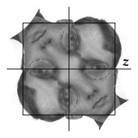
Let's look at a few of the properties of the function
f (
z )=
z2 visible in this figure.
At
z=
i we easily recognize the spot on my right ear
which represents the point
w=−1.
The same spot is found at
z=−
i.
This reflects the fact that
f (
i )=
f ( −
i )=−1.
Similarly,
my mouth, which represents the region near
w=−
i,
is found near the two square roots of −
i,
which are
z=± ( 1 −
i ) / √2.
In fact, every part of my face is found at two places in the
z plane,
except for the spot between my eyes corresponding to
w=0,
which occurs only at
z=0.
The region near that point is "blown up" into the bright blob near
z=0.
This shows that the value of
f (
z ) changes relatively slowly as we move around near
z=0,
which in turn illustrates that the derivative
f ′(
z ) = 2
z is small when
z is small.
Another approach is to color the
w plane according to some mathematical formula.
It is probably impossible to find The Perfect Coloring,
so depending on what aspect of
f one wants to study,
different colorings have to be used.
Several variants have been suggested
(see the references on
the start page).
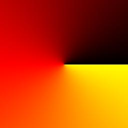
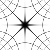
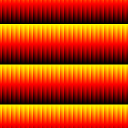
The coloring scheme that I have chosen to use here is built up as follows
(figure
4):
- Choose some color gradient (a smooth sequence of colors) and lay it out "angularly" around w=0.
This lets us identify the argument (angle) arg w by the color.
I have chosen a discontinuous coloring
which makes it easy to find the positive real axis,
and in particular to find the point w=0.
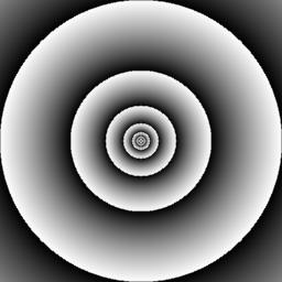
- To keep track of the absolute value | w |,
make a gray-scale mask with brightness (from 0 to 1, with 0 = black) equal to the fractional part of log2 | w | .
This will make it fairly easy to see the direction of growth of | f ( z ) |
(from dark to bright within each ring, the absolute value doubles for each ring).
However, the precise value of | f ( z ) | cannot be seen without some further reference point.
The logarithmic scale counterbalances blow-up effects near multiple zeros.
It also puts zeros and poles on an equal footing,
as we will see below.
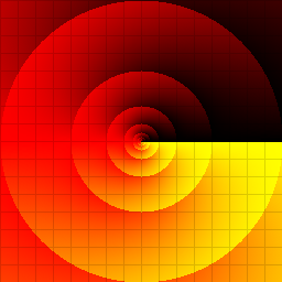
- Blend the two, possibly together with a picture covering some part of the w plane
(for example a picture of a grid, for extra reference).
Figure 4:
The coloring scheme used below.
Colors keep track of arg
w, and shades keep track of |
w |.
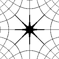
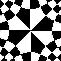
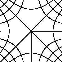
A few words on drawing grids. The first thing that comes to mind is probably something like this:
color
z black if either the real or the imaginary part of
f (
z ) is within some fixed tolerance
from an integer, otherwise color
z white.
This is more or less the same thing as using a picture of a grid superimposed on the
w plane,
just as I used my face in figure
3.
The result is the first image in figure
5,
which obviously isn't very pretty.
The black blob occurs because that grid point happens to be a critical point
of the function (i.e., the derivative is zero).
Conversely, where the function grows quickly, the grid lines become very thin.
A better picture is obtained by interpolating from black to white using gray-scales,
as in the second image.
We still have a black blob, but it looks quite nice,
and it can even be helpful if we want to spot critical points easily.
In case we want all grid lines to be of equal thickness,
the easiest thing is to draw a checkerboard pattern (third image) and run it through an
edge detection filter (fourth image).
In this document, I have used both interpolated and edge-detected grids.
Figure 5:
Grids: plain, interpolated, checkerboard, edge-detected.
f (
z ) =
z2.
4 Case studies of analytic functions
Now we begin our little graphical journey through complex analysis.
Let's recall some basic facts first.
The word
analytic means
expandable in a convergent power series,
which in the complex case turns out to hold for all differentiable functions.
So an analytic function has a power series expansion around each point
z0 :
|
f ( z ) = f ( z0 ) + f ′( z0 ) ( z − z0 ) + |
1
2!
|
f ′′( z0 ) ( z − z0 )2 + … |
|
Assume that
z0 is a zero of
f, so that the first term in the power series vanishes.
Then we have, for
z near
z0,
- f ( z ) ≈ f ′( z0 ) ( z − z0 ), if z0 is a simple zero,
- f ( z ) ≈ [1/2!] f ′′( z0 ) ( z − z0 )2 , if z0 is a double zero,
- f ( z ) ≈ [1/3!] f ′′′( z0 ) ( z − z0 )3 , if z0 is a triple zero, etc.
Consequently, near a zero
z0 of order
k,
f looks very similar to what the monomial
zk
(multiplied by some constant)
looks like near
z=0.
4.1 Monomials
Figure
6 shows the first few
zk.
Recall that complex powers are most easily understood in polar form:
if
z =
R e i ϕ, then
zk =
Rk e i k ϕ.
Try to understand how this can be seen in the pictures!
Also, compare the first two pictures (
k=1 and 2) with figure
3,
which shows essentially the same thing with a different coloring (my face).
Figure 6:
The monomials
f (
z )=
zk for
k=1, 2, 3, 4,
drawn on the square with corners ± 2 ± 2
i.
How are the pictures affected if we multiply by a complex constant?
Figure
7 shows the function
f (
z)=
i z.
As you can see, it looks just like
f (
z )=
z, but rotated −π / 2
(that is, 90 degrees
clockwise; note the minus sign).
This is because multiplication by
i rotates by arg
i = +π / 2
and we are looking at
inverse images;
the points on the negative imaginary axis are mapped by
f to the positive real axis (rotation +π / 2),
so the yellow-black border representing the positive real axis ends up on the negative
imaginary axis in the picture (rotation −π / 2).
Figure 7:
The function
f (
z )=
i z.
Two small exercises:
- What does f ( z )=c z look like, where c is a complex constant?
- And f ( z ) = i z2 ? (Caution: the angle of rotation is not 90 degrees!)
An important thing that we learn from this section is this.
Since f looks like a monomial near its zeros,
a zero z0 of order k can be recognized (with the coloring used here)
by the following features:
- The shaded rings accumulate around z0 .
- If we go in a small circle around z0, the colors cycle k times.
In particular, we cross k times from yellow to black if we go counterclockwise.
(This is our first encounter with the argument principle.)
4.2 A fourth degree polynomial
Let us try all this on a polynomial.
Figure
8 shows the fourth degree polynomial
f (
z ) = (
z + 2 )
2 (
z − 1 − 2
i ) (
z +
i ).
The zeros are clearly visible as the endpoints of the yellow-black borders representing the positive real axis,
and as the points around which the shaded rings of absolute value accumulate.
There are
two yellow-black "spokes" originating from the
double zero at
z = −2
and
one from each of the
simple zeros at
z = 1 + 2
i and
z = −
i.
There are also red spokes, not as sharp, which correspond to (the region near) the negative real axis.
A small enough square around one of the zeros looks,
when magnified, like a rotated version of the pictures of
z2 or
z,
respectively, from figure
6.
Figure 8:
The polynomial
f (
z ) = (
z + 2 )
2 (
z − 1 − 2
i ) (
z +
i ),
drawn on the square with corners ± 3 ± 3
i.
Figure
9 shows the same polynomial,
but with the grid more clearly visible.
This picture illustrates another important feature of analytic functions;
they are
conformal,
which means that
angles are preserved.
More precisely, if two curves intersect at an angle α at the point
z0,
then their images under
f intersect at the same angle α at the point
f (
z0 ).
This is because the tangents of the curves are both rotated by the same angle, namely arg
f ′(
z0 ).
In the picture the phenomenon manifests itself in the reverse direction;
the grid curves intersect orthogonally in the
w plane,
so their inverse images that we see in the
z plane do likewise.
Conformality breaks down at points where the derivative
f ′ is zero
(so-called
critical points of
f ).
Can you find the three points in the picture where something strange seems to happen to the angles?
Those are the three zeros of
f ′ (which is a third degree polynomial in this case).
Figure 9:
The grid represents the square in the
w plane with corners ± 20 ± 20
i,
each square in the grid having side length 2.
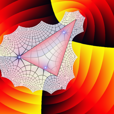
There is a nice little theorem, known as
Lucas' theorem, which states the following:
if
f is a polynomial, then the zeros of
f ′ all lie in the convex hull of the set of zeros of
f.
Figure
10 verifies that this indeed holds in this particular case.
(The
convex hull of a set
M is the smallest convex set containing
M ;
"a rubber band stretched around
M forms the boundary of the convex hull".)
Figure 10:
Lucas' theorem.
The triangle is the convex hull of the zeros of
f.
The three bright spots are the zeros of the derivative
f ′.
4.3 Rational functions
Now to rational functions (quotients of polynomials).
As well as zeros, there are now also
poles - singularities because of zeros in the denominator.
Poles (figure
11) look rather similar to zeros (figure
6), but:
- The colors cycle in the opposite direction
(we cross from black to yellow if we go counterclockwise).
- The absolute value grows to infinity as we approach the pole
(instead of vanishing, as it does for a zero).
Of course, with a different coloring, zeros and poles need not look alike at all!
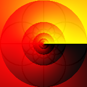
Figure 11:
The functions 1 /
z and 1 /
z2, with a simple and a double pole,
respectively, at
z=0.
Möbius transformations, also known as a
linear fractional transformations,
are rational functions of the form
|
f ( z ) = |
a z + b
c z + d
|
( ad − bc ≠ 0 ). |
|
They have lots of interesting properties,
such as mapping circles to circles
(if we consider straight lines as circles of infinite radius).
Domain coloring perhaps doesn't do justice to all their properties,
but let's look at a few things that can be seen.
Figure
12 shows
f (
z ) = (
z−1 ) / (
z+1 ).
There is a simple zero at
z=1 and a simple pole
z=−1.
The real axis is mapped to the real axis, since
a,
b,
c,
d are all real in this case.
The imaginary axis is mapped to the unit circle,
since
|
| f ( z ) | = |
| z−1 |
| z+1 |
|
= |
distance from z to 1
distance from z to −1
|
, |
|
and the points
z for which these two distances are equal are those on the imaginary axis.
By continuity, the right half plane is mapped to the interior of the unit circle.
Circles containing the point −1 are mapped to circles containing
f ( −1 ) = ∞
(i.e., to straight lines),
as the grid illustrates.
For example, the unit circle is mapped to the imaginary axis.
Figure 12:
The Möbius transformation
f (
z ) = (
z−1 ) / (
z+1 ).
Corners at ± 2 ± 2
i.
Another rational function of some importance is
|
f ( z ) = z + |
1
z
|
= |
z2 + 1
z
|
, |
|
which is shown in figure
13.
There are simple zeros at
z=±
i and a simple pole at
z=0.
The critical points are at
z=± 1.
The real and imaginary axes are mapped to themselves,
as are the right and left half planes.
It is also clearly visible that the unit circle is mapped to the real axis;
in fact,
f (
e iϕ ) =
e iϕ +
e−iϕ = 2 cos ϕ,
by Euler's formula.
Far from the origin, the influence of the term 1/
z is small,
so that
f (
z ) ≈
z (as suggested by the grid).
Figure 13:
The rational function
f (
z ) =
z + 1/
z.
Corners at ± 4 ± 4
i.
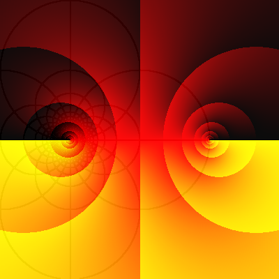
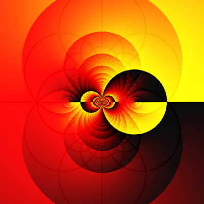
4.4 The argument principle
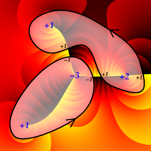
Figure
14 shows a rational function with two simple zeros, one double zero, and one triple pole.
Figure 14:
The function
f (
z ) = (
z − 2 )
2 (
z + 1 − 2
i ) (
z + 2 + 2
i ) /
z3.
Corners at ± 3 ± 3
i.
I will use this to function to illustrate the
argument principle:
Suppose f is analytic (poles are also allowed).
Let γ be a simple closed curve
which does not pass through any zero or pole of f.
Let N (and P) be the number of zeros (poles) of f inside γ,
counted with multiplicity.
Then,
as z goes one lap counterclockwise around γ,
the image curve f ( γ ) winds
N − P times around w = 0.
With our use of colors to keep track of arg
f (
z ),
this is the same as saying that
the colors sweep through the color gradient N − P times as we move around γ.
Counting sweeps (from black through red to yellow) is especially easy with our discontinuous coloring:
jumping from yellow to black adds one,
and jumping from black to yellow subtracts one (since then we are sweeping backwards).
In figure
15 there are two curves which illustrate this.
(You can make up your own curves and try them on any function in this document.)
The upper curve encircles the double zero and one simple zero,
so
N −
P = (2+1) − 0 = 3,
and the number of yellow-to-black crossings is also three.
The lower curve encircles the other simple zero and the triple pole,
so
N −
P = 1 − 3 = −2,
which is OK with the picture since black-to-yellow crossings count as negative.
Figure 15:
The argument principle. Within each curve, the black numbers have the same sum as the blue numbers.
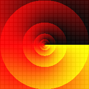
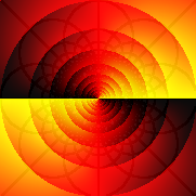
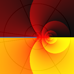
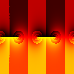
4.5 The exponential and the logarithm
The rather boring first image in figure
16 shows the exponential function
f (
z ) =
ez =
ex ( cos
y +
i sin
y ).
The period 2π
i is clearly visible,
as well as the exponential growth of absolute value from left to right;
recall that |
f | doubles for each shaded band,
so that at the left edge it is very small (
e−10 )
and at the right edge it is very large (
e10 ).
Since the exponential is periodic, it is many-to-one.
Consequently, it is not invertible,
but its restriction to (for example) the strip −π <
y ≤ π is.
The inverse of that particular restriction is called the
principal branch of the logarithm,
and is shown in the second image.
Note the discontinuity at the
branch cut along the negative real axis (colored blue).
The singular point
z=0 is called a (logarithmic)
branch point.
Figure 16:
The exponential
f (
z ) =
ez (corners at ± 10 ± 10
i )
and the logarithm
f (
z ) = log
z (corners at ± 3 ± 3
i ).
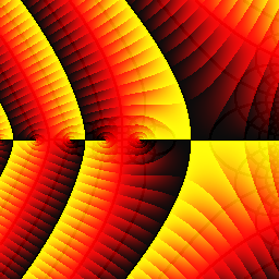
4.6 Trigonometric functions
The trigonometric functions are defined for complex arguments through Euler's formulas
|
cos z = |
eiz + e−iz
2
|
, sin z = |
eiz − e−iz
2i
|
. |
|
Figure
17 shows the complex sine function.
Note the period 2π, the simple zeros at π
n,
and the critical points at π / 2 + π
n (
n integer).
Along the real axis we have the familiar sine wave oscillating between −1 and +1,
but for complex values the sine function is no longer bounded within those limits.
In fact, according to the formula
|
| sin z |2 = sin2 x + sinh2 y |
|
it goes off exponentially in the vertical directions,
as is clearly visible in the picture.
Exercise: Find the points where sin
z = 2.
(Hints:
w = 2 is on the positive real axis,
hence the points we are looking for must lie on some yellow-black border.
We have sin
z = 1 at
z = π / 2 + 2π
n (the yellow-black crossings),
and the absolute value doubles for each shaded band that we pass from dark to bright.
The grid might also be helpful.)
Figure 17:
Three views of the complex sine function
f (
z ) = sin
z.
Corners at ± 10 ± 10
i and ± π ± π
i.
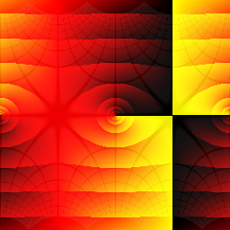
The semi-infinite strip −π / 2 <
x < π / 2,
y > 0 (marked with blue in the third picture)
is mapped to the upper half plane -
I hope you can visualize how the grid can be restored by
bending the two vertical half-lines
x = ± π / 2,
y > 0 down to the real axis
and stretching the region between them accordingly.
By left-right translation and by reflection in the real axis
we obtain similar strips;
where are these strips sent by the sine function?
(If you know about Riemann surfaces, use this to figure out what the Riemann surface for arcsin
z looks like.)
Pictures of the cosine function would look exactly the same except for a translation,
since cos
z = sin (
z + π / 2 ).
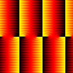
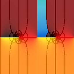
Figure
18 shows two images of the complex tangent function tan
z = sin
z / cos
z,
with period π.
The first picture shows argument and absolute value as usual.
The second one shows argument together with a grid of unit side length,
the region colored blue being mapped into the square with corners 0, 1,
i, 1+
i.
For tan
z all the action takes place near the real axis,
with simple zeros at π
n and
simple poles at π / 2 + π
n.
Some distance away from the real axis, the function is nearly constant
(+
i in the upper half plane, −
i in the lower half plane):
|
tan ( x + i y ) = |
tan x + i tanh y
1 − i tan x tanh y
|
→ |
tan x ± i
1 − (± i tan x )
|
= ± i, y → ± ∞. |
|
The lines
x = π / 4 and
x = −π / 4 are mapped to the
right and left part of the unit circle, respectively.
Figure 18:
Complex tangent function
f (
z ) = tan
z.
Corners at ± π ± π
i.
4.7 Essential singularities
If
f (
z ) is known to be analytic in some disc (the interior of a circle)
D,
except maybe at the center
z0,
then there are three possible cases:
- f ( z ) is bounded near z0, in which case it is actually analytic there, and hence in all of D.
(Riemann's removable singularities theorem.)
- f ( z ) is unbounded near z0, but ( z − z0 )k f ( z ) is analytic for some k > 0.
Then z0 is called a pole of order k.
- Neither of the above. Then z0 is called an essential singularity.
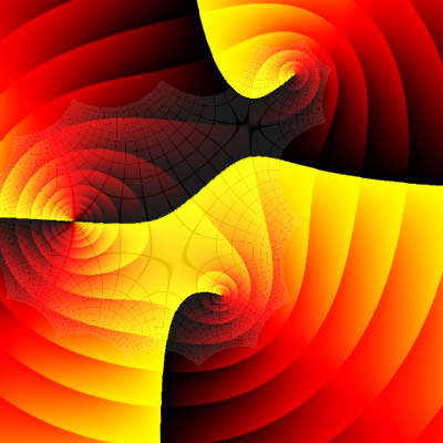
Figure
19 shows a function with an essential singularity at the origin.
Clearly, some fairly complicated stuff seems to be going on near the singularity!
Maybe we could get a better view if we zoomed in a bit?
No, in fact that wouldn't help much, because of the remarkable
Picard's great theorem (there is also a Picard's little theorem):
In any disc with center at the essential singularity z0,
no matter how small,
f assumes all (or possibly all but one) complex values.
Figure 19:
f (
z ) = sin ( 1 /
z ).
Corners at ± 1 ±
i.
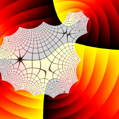
4.8 The maximum principle
You may have noticed a curious thing about the shading that I use to indicate
the absolute value of functions:
if some band forms a closed curve ("a shaded ring"), then there is always at least one zero
or singularity inside.
In fact, we recognize zeros and poles as points where shaded rings "gather round".
This is a manifestation of
the maximum principle, which says (briefly):
If f is analytic, then | f | has no local maxima.
A more precise statement is the following:
Let M be a domain (an open connected set) in the complex plane,
and suppose that f is analytic in M (no singularities allowed!).
Then | f | has no maximum value in M, except in the trivial case that f is constant.
If
f has no zeros in
M, then 1/
f is analytic in
M and has no maximum,
which implies that |
f | has no
minimum in
M either.
(But if
f has zeros in
M, then they are of course minima of |
f |.)
Another corollary is that if
M is bounded,
and
f extends continuously out to the boundary of
M,
then |
f | attains its maximum on the boundary
(and its minimum too, if
f has no zeros in
M).
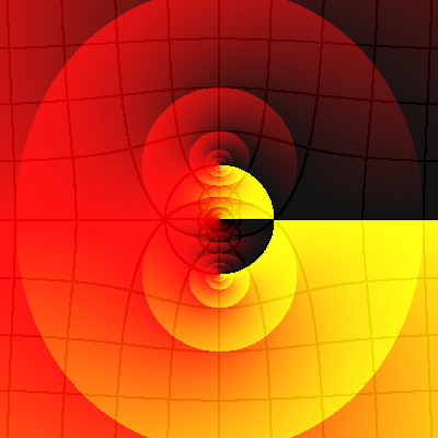
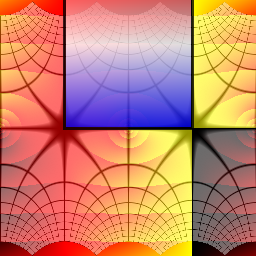
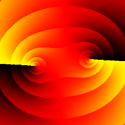
4.9 The gamma function
I will close this little tour with a look at a less common function, namely the gamma function Γ,
which is defined by
|
Γ( z ) = | ⌠
⌡
|
∞
0
|
t z−1 e−t dt. |
|
This integral is convergent only for
z in the right half plane,
but the gamma function can be
analytically continued to the left half plane as well,
using the property Γ(
z + 1 ) =
z Γ(
z )
(which is easily proved using integration by parts).
For example, Γ( −0.1 ) is defined to be Γ( −0.1 + 1 ) / 0.1 = 10 Γ( 0.9 ),
where Γ( 0.9 ) is already defined by the integral above,
and so on.
This works fine unless
z is zero or a negative integer,
since then we are eventually forced to divide by zero;
the gamma function has simple poles at these points.
For nonnegative integers
n we have Γ(
n + 1 ) =
n! ,
so that the gamma function is a continuous version of
n-factorial.
Another exactly known value is
Γ( 0.5 ) = √{π}.
Figure 20:
The gamma function Γ(
z ).
Corners at ± 4 ± 4
i.
5 Iteration of functions
You may have tried the following on your pocket calculator sometime:
type in an arbitrary positive number, and then push the "square root" button over and over.
(This is called
iterating the square root function.)
If you start with a number greater than 1, it will become smaller for each key-press,
until it is so close to 1 that the calculator thinks that is actually
is 1.
Similarly, if you start with a number between 0 and 1,
the sequence will approach 1 from below.
Pushing some other button, for example "cos", leads to less obvious (and more interesting) results.
Even more interesting things happen when we go into the complex plane and iterate analytic functions.
The notation
f(n)(
z ) is used to denote the
n-th iterate of
f,
that is,
|
f(1)( z ) = f ( z ), f(2)( z ) = f ( f ( z ) ), f(3)( z ) = f ( f ( f ( z ) ) ), |
|
and so on.
5.1 Quadratic polynomials
The most well-known case is when
f is a quadratic polynomial.
For example, let
f (
z ) =
z2 +
c, where
c = −0.75 − 0.2
i.
Figure
21 shows the first four iterates:
| |
|
| |
| |
|
|
f(2)( z ) = ( z2 + c )2 + c = z4 + 2 c z2 + c2 + c |
| |
| |
|
|
f(3)( z ) = ( z4 + ... )2 + c = z8 + ... |
| |
| |
|
| f(4)( z ) = ( z8 + ... )2 + c = z16 + ... |
| |
|
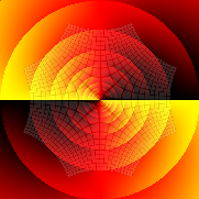
The degree doubles at each step, so likewise does the number of zeros.
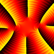
Figure 21:
The iterates
f(n)(
z ) for
n=1, 2, 3, 4,
where
f (
z ) =
z2 − 0.75 − 0.2
i.
Corners at ± 2 ± 2
i.
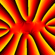
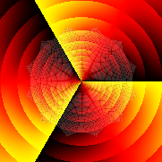
Figure
22 depicts the function obtained by iterating
f twenty times.
This function is a polynomial of degree 2
20,
so it has 2
20 = 1048576 zeros!
About a hundred of them can be distinguished in the picture
(
here is a larger picture).
The black region is not really supposed to be there -
it consists of the points where an overflow error occurs
because the value of the function is too large to represent
with standard precision floating point arithmetic.
However,
for large
z the behaviour of the function is dominated by the
contribution from the leading term
z1048576,
which is a monomial,
so by now you should be able to figure out what
the function will eventually look like if we zoom out enough,
even if we can't
compute it without some special software.
Figure 22:
The twentieth iterate
f(20)(
z ), where
f (
z ) =
z2 − 0.75 − 0.2
i.
Corners at ± 1.6 ± 1.1
i.
What happens when we iterate this polynomial further?
It is not hard to realize that
f(n)(
z ) → ∞ as
n → ∞
if, for example, |
f(k)(
z ) | > 2 for some
k,
since after that the absolute value will keep increasing.
This holds of course if
z is one of the black overflow points,
and actually for most other
z as well.
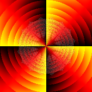
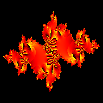
Those
z for which
f(n)(
z ) does
not tend to infinity
constitute
the filled Julia set of
f,
which is shown in figure
23.
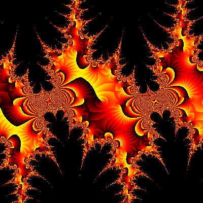
Actually, the Julia set here consists of "fractal dust" hidden deep inside the bright
"islands" in the picture, so what we see is rather the complement of the Julia set.
Colors indicate rate of divergence;
for greenish points the iterates
f(n)(
z )
become very large already after a few steps
(compare with the black overflow region in figure
22),
for reddish points the iterates diverge more slowly.
Figure 23:
The filled Julia set of
f (
z ) =
z2 − 0.75 − 0.2
i.
For other values of
c, the behavior of the iterates can be quite different.
When varying
c and investigating the iterates of
fc (
z ) =
z2 +
c,
one obtains the famous Mandelbrot set,
which contains those
c for which
fc(n) ( 0 ) does not diverge to infinity.
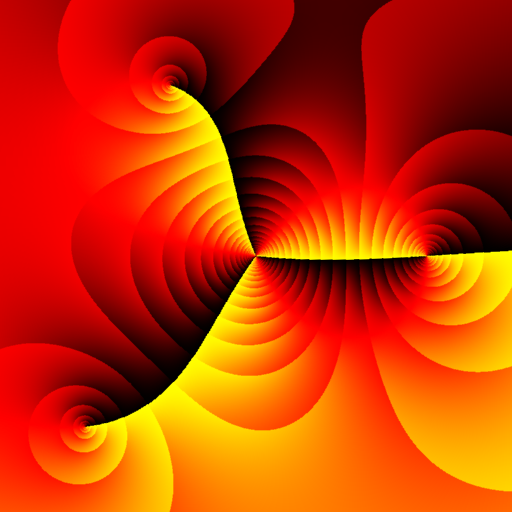
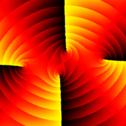
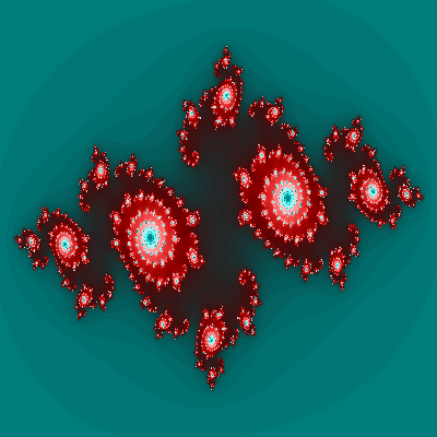
5.2 A sine function
Iterating other functions can also produce nice pictures.
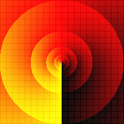
Figure
24 shows an example.
Figure 24:
The fifth iterate
f(5)(
z ) of
f (
z ) = ( 1 +
i ) sin
z.
Corners at ± 3 ± 3
i.
6 Want to learn more?
On the
the start page you will find pointers to more information.
File translated from
TEX
by
TTH,
version 4.10.
On 10 Oct 2017, 12:39.